The phovafer Package
introduction.RmdIntroduction
Despription
“PHOtoVoltAic FindER” (phovafer) is developed for identifying the solar photovoltaic (PV) users among the regular consumers in the low-voltage network. It contains the R functions for data representation, feature extraction, and PV users’ classification using the extracted features.
Load the package
library(phovafer)
#> Loading required package: caret
#> Loading required package: lattice
#> Loading required package: ggplot2
#> Loading required package: matrixStatsFunctions
load.daily( )
Represent multiple days of smart meter reading vector (or load vector) of one household as one matrix with each row presents the daily observations. The following example shows how to transform the vector that contains three months smart readings of household “X1” into a matrix with each row presents a daily load profile.
# Import the load profiles.
data("loadsample")
# Get the load profile matrix of the household X1.
loadsample.X1<-load.daily(loadsample$X1, load.date=loadsample$date, num.obs=48)
plot(loadsample$time[1:48], loadsample.X1[1, ], ylim = range(loadsample.X1), type="l", xlab = "Time", ylab="Load")
for (i in 2:nrow(loadsample.X1)){
lines(1:48, loadsample.X1[i, ], col=sample(10))
}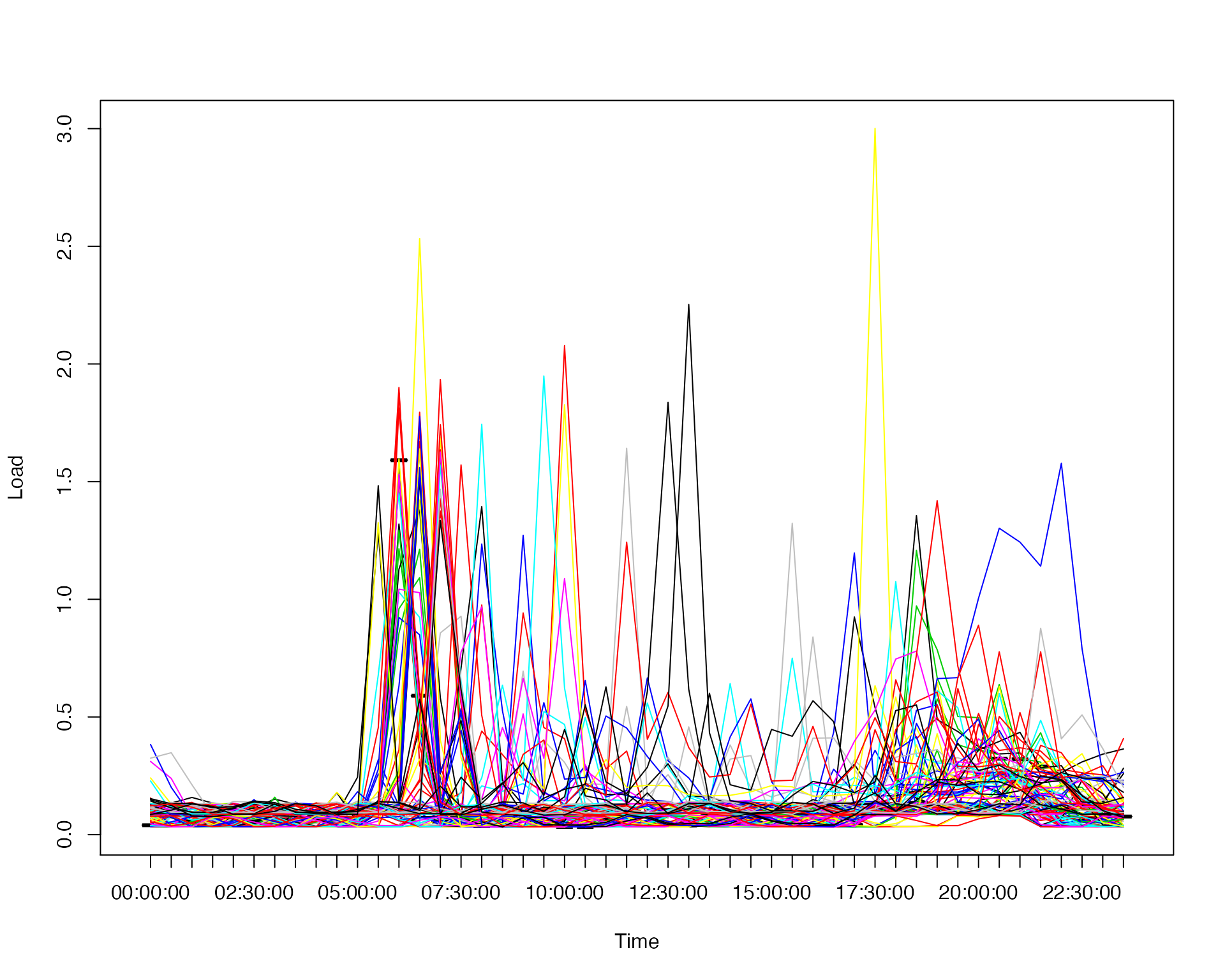 ## features.load( ) Extract the features from the load profiles of each household. These features are prepared for identifying the prosumers and regular consumers. There are 63 features extracted in total. The following code gives an example for how to extract the features from the three months smart meter readings of household “X1”.
# Import the load profiles.

data("loadsample")

# Get the load profile matrix of the household X1.

loadsample.X1<-load.daily(loadsample$X1, load.date=loadsample$date, num.obs=48)

# Compute the features.

features.X1<-features.load(loadsample.X1, unique(loadsample$week), mor.be=13, aft.be=39)
summary(features.X1)
#>                 Length Class  Mode
#> output.features 63     -none- numeric
#> features.name   63     -none- character
features.importance( )
Compute the importance values of the features that identify PV and non-PV consumers based on the p-values of Kruskal test. An example to compute the degree of difference of each feature between the PV users and regular consumers is shown below:
# Load the smart meter readings and the simulated PV generations.

data("loadsample")
data("pvSample")

# Get the load profiles of both PV and non-PV consumers.

N.house<-ncol(loadsample[,-c(1:6)]) # N.house is the total number of households.

NPV.day<-lapply(loadsample[,-c(1:6)], load.daily, load.date=loadsample[,1], num.obs=48)

# Assuming 30% of the households use PV. Generate the PV samples.

perc=0.3
pv.house<-floor(N.house*perc) # The total number of households that use PV.
M<-ncol(pvSample[,-c(1:6)])
pv.rand<-sample(1:M, pv.house, replace = TRUE, prob = rep(1/M, times=M))
pvSample<-cbind(pvSample[ ,c(1:6)], pvSample[ ,-c(1:6)][ ,pv.rand]) # Generated new PV generation samples.

date.PV.NPV<-unique(pvSample$date)
PV.day<-lapply(pvSample[,-c(1:6)], load.daily, load.date=pvSample$date, num.obs=48)

house_pv<-sample(N.house)[1:pv.house] # Randomly selected PV households.

# Compute the real load demand of the PV consumers using the smart meter reading (loadsample),
# and the simulated PV samples (pvSample).

demand_pv<-vector(mode = "list", length = length(PV.day))

for (k in 1:pv.house){
   demand_pv[[k]]<-NPV.day[[house_pv[k]]]-PV.day[[k]]
}
demand_npv<-NPV.day[-house_pv]

# Label the PV consumers with 0, and non-PV consumers with 1.

label.PV<-c(rep(0, times=length(house_pv)),
          rep(1, times=length(demand_npv)))
label.PV<-factor(label.PV)

# Extract the features used to identify PV and non-PV users.

date.week<-weekdays(as.Date(date.PV.NPV))
x.week<-date.week
mor.be<-13 # It presents 06:00:00.
aft.be<-39 # It presents 19:00:00.

feature.PV<-lapply(demand_pv, features.load, x.week, mor.be, aft.be)
feature.NPV<-lapply(demand_npv, features.load, x.week, mor.be, aft.be)

# Get the name of the features.

features.name<-feature.PV[[1]]$features.name # Get the name of the computed features.

# Prepare the feature matrix.

feature.PV.new<-feature.PV[[1]]$output.features
for (i in 2:length(feature.PV)){
  feature.PV.new<-rbind(feature.PV.new, feature.PV[[i]]$output.features)
}

feature.NPV.new<-feature.NPV[[1]]$output.features
for (i in 2:length(feature.NPV)){
  feature.NPV.new<-rbind(feature.NPV.new, feature.NPV[[i]]$output.features)
}

# Compute the significance of each feature and select the 12 most significant features.

feature.PV.NPV<-rbind(feature.PV.new, feature.NPV.new)

p.Spring<-apply(feature.PV.NPV, 2, features.importance, label.PV)

p.Spring
#>  [1] 6.408487e-87 4.297502e-28 6.408268e-87 5.758549e-83 6.408487e-87
#>  [6] 4.715540e-61 6.725437e-87 1.016897e-73 6.408268e-87 2.666825e-85
#> [11] 6.408487e-87 9.054134e-61 6.408080e-87 1.903240e-66 1.886922e-86
#> [16] 2.321602e-74 6.408205e-87 1.146392e-10 4.774787e-43 7.521437e-41
#> [21] 3.072226e-77 6.408487e-87 4.297502e-28 6.408268e-87 5.758549e-83
#> [26] 6.408487e-87 4.715540e-61 6.725437e-87 1.016897e-73 6.408268e-87
#> [31] 2.666825e-85 6.408487e-87 9.054134e-61 6.408080e-87 1.903240e-66
#> [36] 1.886922e-86 2.321602e-74 6.408205e-87 1.146392e-10 4.774787e-43
#> [41] 7.521437e-41 3.072226e-77 6.408487e-87 4.297502e-28 6.408268e-87
#> [46] 5.758549e-83 6.408487e-87 4.715540e-61 6.725437e-87 1.016897e-73
#> [51] 6.408268e-87 2.666825e-85 6.408487e-87 9.054134e-61 6.408080e-87
#> [56] 1.903240e-66 1.886922e-86 2.321602e-74 6.408205e-87 1.146392e-10
#> [61] 4.774787e-43 7.521437e-41 3.072226e-77
classify.pv.npv( )
Identify PV and non-PV consumers using a set of linear classifiers, i.e., Naive Bayesian, Support Vector Machine, Generalized Linear Model, Linear Discriminate Analysis and Perceptron. An example for identifying PV and non-PV consumers based on their load profile in Spring is given as follows:
# Load data.

data("loadsample")
data("pvSample")
#######################################################
## Get the load profiles of both PV and non-PV consumers.

N.house<-ncol(loadsample[,-c(1:6)]) # N.house is the total number of households.

NPV.day<-lapply(loadsample[,-c(1:6)], load.daily, load.date=loadsample[,1], num.obs=48)

# Assuming 30% of the households use PV. Generate the PV samples.
# Remark that in a real experiment there should be hundreds or thousands of simulation replication.
# Only one replication is shown below for the instant instruction.

perc=0.3
pv.house<-floor(N.house*perc)
M<-ncol(pvSample[,-c(1:6)])
pv.rand<-sample(1:M, pv.house, replace = TRUE, prob = rep(1/M, times=M))
pvSample<-cbind(pvSample[ ,c(1:6)], pvSample[ ,-c(1:6)][ ,pv.rand])

date.PV.NPV<-unique(pvSample$date)
PV.day<-lapply(pvSample[,-c(1:6)], load.daily, load.date=pvSample$date, num.obs=48)

house_pv<-sample(N.house)[1:pv.house] # Randomly select the PV households.

# Compute the real load demand of the PV consumers using the smart meter reading (loadsample), # and the simulated PV samples (pvSample).

demand_pv<-vector(mode = "list", length = length(PV.day))

for (k in 1:pv.house){
  demand_pv[[k]]<-NPV.day[[house_pv[k]]]-PV.day[[k]]
}
demand_npv<-NPV.day[-house_pv]

# Label the PV consumers with 0, and non-PV consumers with 1.
label.PV<-c(rep(0, times=length(house_pv)),
            rep(1, times=length(demand_npv)))
label.PV<-factor(label.PV)

############ Prepare the features used to identify PV and non-PV users.
date.week<-weekdays(as.Date(date.PV.NPV))
x.week<-date.week
mor.be<-13
aft.be<-39

feature.PV<-lapply(demand_pv, features.load, x.week, mor.be, aft.be)
feature.NPV<-lapply(demand_npv, features.load, x.week, mor.be, aft.be)

features.name<-feature.PV[[1]]$features.name # Get the name of the computed features.

# Prepare the feature matrix.
feature.PV.new<-feature.PV[[1]]$output.features
for (i in 2:length(feature.PV)){
  feature.PV.new<-rbind(feature.PV.new, feature.PV[[i]]$output.features)
}

feature.NPV.new<-feature.NPV[[1]]$output.features
for (i in 2:length(feature.NPV)){
  feature.NPV.new<-rbind(feature.NPV.new, feature.NPV[[i]]$output.features)
}

##### Compute the significance of each feature and select the 12 most significant features.

feature.PV.NPV<-rbind(feature.PV.new, feature.NPV.new)

p.Spring<-apply(feature.PV.NPV, 2, features.importance, label.PV)

p.Spring<-sort(p.Spring, decreasing = FALSE, index.return=TRUE)
features.order<-features.name[p.Spring$ix]

PV_feature<-feature.PV.new[,p.Spring$ix[1:12]]
NPV_feature<-feature.NPV.new[ ,p.Spring$ix[1:12]]

##### Visualize the differences of between the features of PV and non-PV consumers.
##### Top 5 features are selected for example.

PV.NPV<-data.frame(rbind(PV_feature[,1:5], NPV_feature[,1:5]))
PV.NPV$cls<-label.PV

PV.NPV<-PV.NPV[sample(nrow(PV.NPV)), ]

PV.NPV$cls<- factor(PV.NPV$cls, levels = c(0,1), labels = c("PV", "non-PV"))
ggpairs(PV.NPV, title="The 5 most significant features",
        mapping=ggplot2::aes(colour = cls))
#> `stat_bin()` using `bins = 30`. Pick better value with `binwidth`.
#> `stat_bin()` using `bins = 30`. Pick better value with `binwidth`.
#> `stat_bin()` using `bins = 30`. Pick better value with `binwidth`.
#> `stat_bin()` using `bins = 30`. Pick better value with `binwidth`.
#> `stat_bin()` using `bins = 30`. Pick better value with `binwidth`.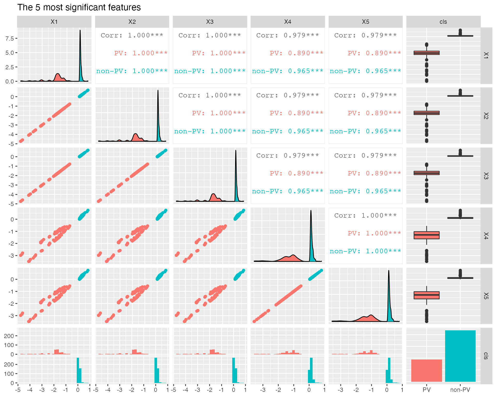
######### Use the above selected features to classify PV and non-PV consumers.

#### Prepare the training and testing dataset.

set.seed(123)

# 70% of the data (PV and non-PV) are used for training, and the remainder are used for testing.

train.data<-0.7
# Prepare the training and testing datasets of PV consumers.
n.pv<-sample(nrow(PV_feature))
data.train.pv<-as.matrix(PV_feature[n.pv[1:floor(train.data*length(n.pv))], ])
data.test.pv<-as.matrix(PV_feature[n.pv[-c(1:floor(train.data*length(n.pv)))], ])

pv.cls.test<-rep(0, times=nrow(data.test.pv))
pv.cls.train<-rep(0, times=nrow(data.train.pv))

# Prepare the training and testing datasets of non-PV consumers.

n.npv<-sample(nrow(NPV_feature))
data.train.npv<-as.matrix(NPV_feature[n.npv[1:floor(train.data*length(n.npv))], ])
data.test.npv<-as.matrix(NPV_feature[n.npv[-c(1:floor(train.data*length(n.npv)))], ])

npv.cls.test<-rep(1, times=nrow(data.test.npv))
npv.cls.train<-rep(1, times=nrow(data.train.npv))

### Composite the training dataset.

data.train<-as.data.frame(rbind(data.train.pv, data.train.npv))
data.train$cls<-c(pv.cls.train, npv.cls.train)
data.train$cls<-factor(data.train$cls, levels = c(0,1), labels = c("False", "True"))

### Composite the testing dataset.

data.test<-as.data.frame(rbind(data.test.pv, data.test.npv))
data.test$cls<-c(pv.cls.test, npv.cls.test)
data.test$cls<-factor(data.test$cls, levels = c(0,1), labels = c("False", "True"))

# 5-Fold cross-validation is used for model selection.

classify.results<-classify.pv.npv( data.train,
                                   data.test,
                                   trControl=trainControl(method='cv',number=5))

# Print the testing reults.

classify.results
#> $model.name
#> [1] "Naive Bayesian"               "Support Vector Machine"
#> [3] "Generalized Linear Model"     "Linear Discriminate Analysis"
#> [5] "Perceptron"
#>
#> $results
#> [1] 1.0000000 1.0000000 1.0000000 0.9893048 1.0000000
Acknowlegement
This package is developed for the project “Analytical Middleware for Informed Distribution Networks (AMIDiNe)” (EPSRC Reference: EP/S030131/1). The developers would like to thank for the help from Bruce Stephen, Jethro Browell, Rory Telford, Stuart Galloway, and Ciaran Gilbert from the University of Strathclyde.